By Ben Crabb, Regional Economist
(March 10, 2022) Utah’s employment landscape is variable and dynamic. Employment levels and the size of industrial sectors differ across the state’s 29 counties.
To understand the nuances of Utah’s labor force, economists use a handful of data tools to understand the workforce. These tools include the North American Industry Classification System (NAICS), NAICS supersectors, percent employment in each supersector for each Utah county, location quotients, and the Hachman Index of industrial diversification.
This information helps policymakers understand these nuances and is important in making informed decisions.
Below is a brief overview of employment levels and the dominance of each industrial sector across the state.
North American Industry Classification System (NAICS)
When you hear about jobs data, you often hear about gains or losses in different industrial sectors, like leisure and hospitality, or manufacturing. These industry sectors are based on the North American Industry Classification System (NAICS) which categorizes business establishments based on the type of work they do. Economists can then summarize job counts based on NAICS classes, providing insight into the employment & industrial characteristics of national, state, and local economies.
At the top of the NAICS classification pyramid are broad “supersector” categories. These are commonly used to provide a high-level overview of economic dynamics. The supersector/sector groupings are:
Natural Resources and Mining (supersector; NAICS Sector Codes 11-21)
Construction (sector; NAICS 23)
Manufacturing (sector; NAICS 31-33)
Trade, Transportation, and Utilities (supersector; NAICS 42-49 and 22)
Information (sector; NAICS 51)
Financial Activities (supersector; NAICS 52-53)
Professional and Business Services (supersector; NAICS 54-56)
Education and Health Services (supersector; NAICS 61-62)
Leisure and Hospitality (supersector; NAICS 71-72)
Other Services (sector; NAICS 81)
Government / Public Administration (sector; NAICS 92)
Proportion of overall employment by sector
The proportion of overall employment across these supersectors varies by geographic region based on differences in historical development, demographics, and geography. For example, in Las Vegas, a significant proportion of employment is in the Leisure and Hospitality sector. In New York City a large proportion of employment is in the Financial sector.
Similarly, variations in employment structure are seen at local and county levels. In Utah, the metropolitan Wasatch Front region has a diversified economy with employment spread across a broad range of industries. In the Uinta Basin, however, employment is more concentrated in Mining and oil and gas extraction. In southern Utah, Leisure and Hospitality employment leads due to considerable tourism.
These regional variations are shown below in Figure 1, which maps the percent of county employment that falls into each of the 11 supersector categories:

Figure 1. Percent employment by county and sector, September 2021. Employment levels above 20% are labeled.
Location Quotients
We see that the employment share in different sectors varies noticeably by geography. But just knowing the employment proportion in sector X for county Y doesn’t tell us anything about county Y’s relative dependence on sector X compared to what might be expected. For example, we know that 6.7% of jobs in Salt Lake County are in the construction sector. But compared to most counties, is 6.7% relatively high, low, or pretty average? To answer this we need to compare local area employment shares against a larger reference region.
This is where the concept of the “Location Quotient” (LQ) comes in handy. LQ’s compare a local area’s industry sector prevalence against a larger reference region. Put another way, LQ’s measure the relative concentration of a given sector or industry in a given place.
Higher LQ’s indicate greater specialization. Lower LQ’s indicate lesser specialization or perhaps a deficiency. A location quotient of 1.0 for a particular sector means that local employment in that sector has the same prevalence as it does in the larger reference region. In this article, we used the nation as the reference region.
Here’s an example: if manufacturing made up 10% of the nation’s employment, and in Weber County manufacturing also made up 10% of the county’s employment base, then the location quotient for manufacturing in Weber County would be 1.0 (10%/10%). If 20% of jobs in Weber County, however, are in the manufacturing sector, then the location quotient for manufacturing in Weber County would be 2.0 (20%/10%), indicating that manufacturing is twice as prevalent to Weber County’s local employment than it is to the nation as a whole. Alternatively, if only 5% of jobs in Weber County were in manufacturing, then the location quotient would be 0.5, indicating that manufacturing is only half as important in Weber County as to the nation as a whole.
As a rule of thumb, an LQ value of 1.2 or higher indicates some degree of industry-sector specialization, and an LQ value of 0.8 or lower indicates that a region may be underrepresented in that industry.
In small regions, LQ’s can be somewhat problematic due to the large effect that only a few firms may have on the values. For example, Piute and Daggett counties are so small that their location quotients should be interpreted with extreme caution.
The next few maps show LQ's for the 11 supersectors in each of Utah's 29 counties. Because the mining sector has a few counties with extreme LQ's greater than 10, it is shown on a separate map in Figure 2. County LQ's for the other 10 supersectors fall into a more typical range of values, and are shown in Figure 3.
Location Quotients: Mining Sector. The prevalence of the Natural Resources and Mining Sector in a locality is highly dependent on that locality’s natural endowment. For areas with large deposits of oil and gas, specialization in this sector can be extreme compared to the national average. For example, in Utah the Uinta Basin overlays oil and gas deposits. In Figure 2 we see that LQ’s for the Natural Resources and Mining sector in Duchesne, Uintah, Carbon, and Emery counties all exceed 20, indicating that those counties have more than twenty times the employment concentration in the Natural Resources and Mining sector than the national average! This is how regions get labeled with monikers like “energy belt” or “energy basins.”

Figure 2. Location Quotient (LQ) values for the Natural Resources and Mining Supersector, September 2021. Counties in the Uinta Basin have a high degree of specialization in this sector.
Location Quotients: All other sectors. Outside of the Natural Resources & Mining sector, the other supersectors don’t exhibit such significant LQ values. But there are still very large LQ values for several sectors in some Utah counties. Notably, the Leisure and Hospitality sector provides jobs at a rate 3-5x the national average in southern Utah counties that are home to national parks. We can also see that the Construction sector is an area of specialization in fast-growing Morgan, Washington, and Wasatch counties. Furthermore, Manufacturing is an area of specialization in several counties — Cache, Box Elder, and Juab — on the periphery of the Wasatch Front.
Figure 3 shows LQ’s by industry sector for each county to help visualize the spatial distribution of industry importance across Utah.
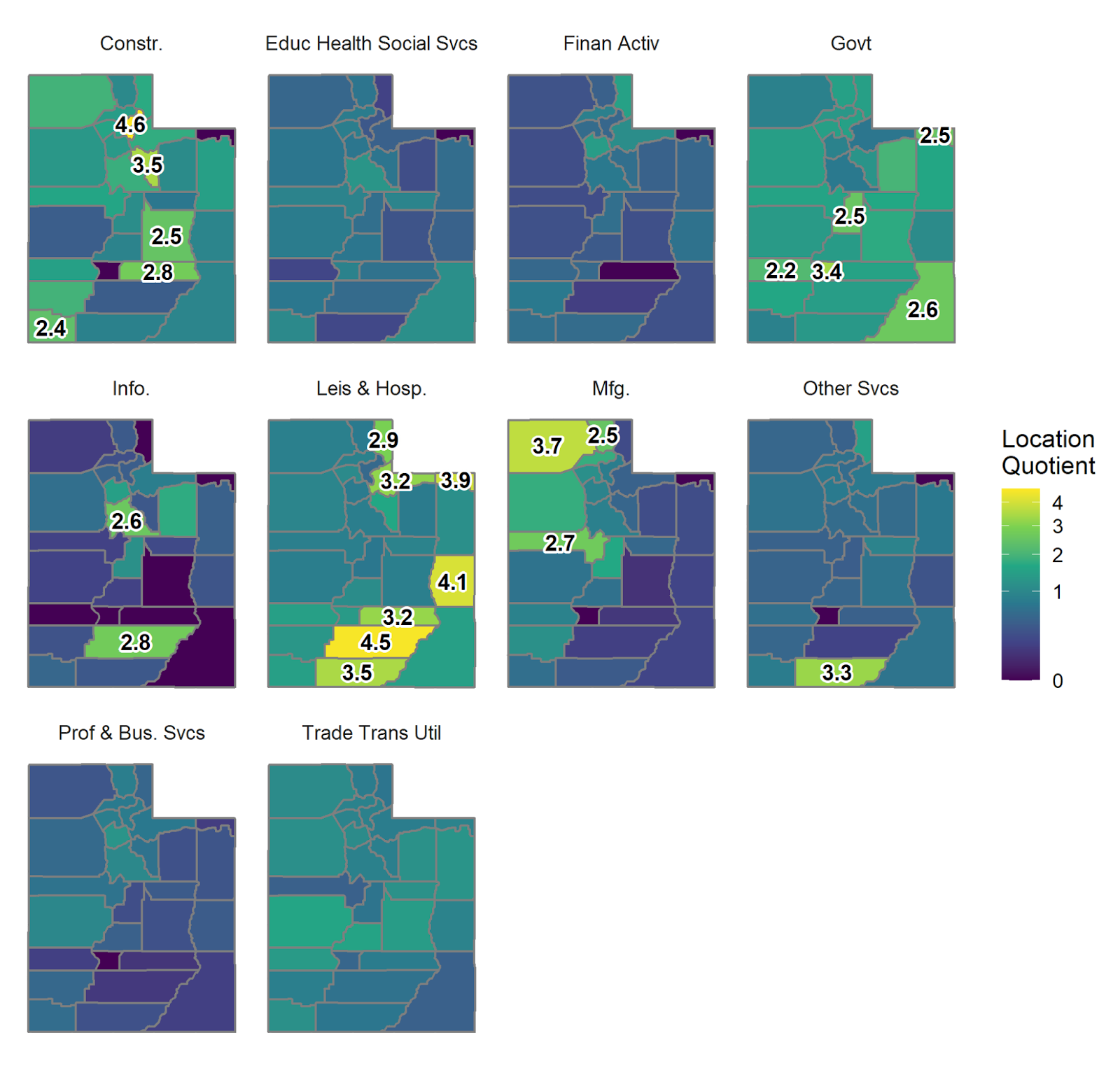
Figure 3. Location Quotient (LQ) values per supersector, excluding Natural Resources & Mining, for Utah Counties, September 2021. LQ’s greater than two are labeled.
The Hachman Index
Now that we have an idea of sector-specific employment concentrations for each county, we find ourselves wishing for a way to measure the overall character of a county’s industrial landscape. Is this a county of overall specialization, or of industrial diversity? Counties with greater diversification tend to have greater resilience against economic downturns that may initiate from a particular sector. A diverse industrial composition tends to help develop and attract a diverse workforce. This dynamic can contribute to a virtuous cycle of investment, growth and resilience. On the other hand, counties with specialization in just a few sectors can be subject to stormier up-or-down economic swings. Low diversification is not a guarantee of economic deficiency. Instead it speaks to a higher degree of economic variability and vulnerability in a regional economy.
In any case, there are metrics for measuring a local economy’s industrial diversity. Among the more well-known is the Hachman Index. This index establishes a diversification scale between 0 and 100. A value of 100 indicates diversification equal to the larger reference region, with lesser values indicating a descending degree of economic diversity. The index values are calculated by taking a weighted sum of a local area’s industry LQ values (where weights are equal to the employment share of each industry) and then taking the reciprocal of that summation:

Hachman Index = 1 / (i(ESi/ERi) x ESi)
where
ESi is employment share of industry i in the area of interest.
ERi is employment share of industry i in the reference region.
To provide context to the Hachman Index values shown below, the top 10 Index values from 2018 for states were all above 93 (compared to a score of 100 for the nation). The bottom 10 states had Hachman Index values below 68. These 2018 values are taken from a publication by the Kem C. Gardner Institute at the University of Utah that also assessed county Hachman Index values for Utah in that year: https://gardner.utah.edu/wp-content/uploads/Hachman-Brief-Apr2020.pdf. (The Gardner Institute publication used 2-digit NAICS codes instead of supersectors, meaning they used around 20 industrial categories instead of 11, but their results are similar to those reported here.)
Hachman Index values for each Utah county are shown in Figure 4. Some predictable patterns are evident. Large Wasatch Front counties have the highest Hachman Index values. Salt Lake County, Utah’s largest, has a Hachman Index value of 95. This indicates its economy is highly diversified. Duchesne and Uintah counties, with their large dependence on the oil & gas industry, have Utah’s lowest Hachman Index values at only 14 and 26, respectively. This speaks to extreme economic concentration.
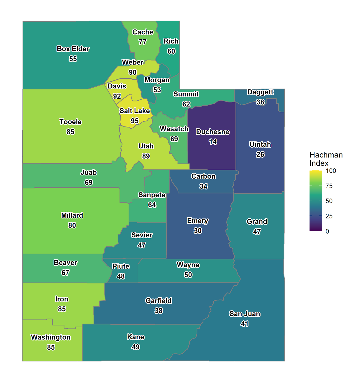
Figure 4. Hachman Index values of industrial diversification for Utah counties, September 2021. Reference region: USA (Hachman = 100). The Hachman Index value for the State of Utah was 97.6.
Conclusion
The industrial and employment landscape of Utah counties varies considerably across the state. Using location quotients and the Hachman Index of industrial diversity, we can see that the metropolitan counties of the Wasatch Front have highly diversified economies with employment spread out across many industrial sectors. Conversely, the energy-producing counties of the Uintah Basin and the tourism-dependent counties of southern Utah have less diverse economies with greater specialization in a few industrial sectors in which they have a competitive advantage over other regions.
While industrial specialization can be a strong basis for economic development, it also renders an area more vulnerable to potential economic woes should the fortunes of a few industries take a downward turn. For example, employment losses in the early months of the COVID pandemic were more extreme in the leisure and hospitality-dependent counties of southern Utah than they were in most other counties in the state. On the other hand, industrial diversification tends to be associated with stronger long term growth and can buffer a local economy from the highs and lows of any particular industry or small group of industries. Much like diversified financial portfolios, diversified local economies tend to outperform concentrated local economies in the long run.
Tables with employment metrics
The two tables below provide the numbers that went into the maps above. In addition to values for every county, the tables also contain the metrics for the State of Utah as a whole. The data can be sorted for any of the columns, allowing you to quickly see the top or bottom counties per sector.
Table 1 shows the proportion of total employment per NAICS supsersector.
Table 2 shows location quotient (LQ) values and the Hachman Index value.
Table 1: Proportion of employment per sector
Area | Total jobs Sep 2021 | Mining | Constr. | Mfg. | Trade Trans Util | Info. | Finan Activ | Prof & Bus. Svcs | Educ Health Social Svcs | Leis & Hosp. | Other Svcs | Govt |
United States | 147328000 | 0.4 | 5.0 | 8.4 | 18.9 | 2.0 | 6.0 | 14.5 | 16.1 | 9.9 | 3.7 | 15.0 |
State of Utah | 1627876 | 0.6 | 7.6 | 9.0 | 18.8 | 2.6 | 6.0 | 14.4 | 13.3 | 9.4 | 2.6 | 15.6 |
Salt Lake County | 752312 | 0.4 | 6.7 | 7.8 | 20.1 | 2.9 | 8.4 | 17.9 | 11.5 | 7.8 | 2.9 | 13.7 |
Utah County | 291619 | 0.1 | 9.3 | 7.4 | 16.9 | 5.1 | 4.5 | 14.7 | 20.2 | 8.3 | 2.1 | 11.5 |
Davis County | 136580 | 0.1 | 7.9 | 9.6 | 17.4 | 1.0 | 3.4 | 12.2 | 13.4 | 10.3 | 2.8 | 22.0 |
Weber County | 114481 | 0.0 | 7.1 | 15.2 | 17.3 | 0.5 | 5.2 | 11.2 | 12.9 | 8.7 | 2.5 | 19.3 |
Washington County | 78056 | 0.6 | 11.9 | 5.1 | 21.9 | 1.0 | 3.8 | 8.6 | 16.4 | 14.4 | 3.0 | 13.2 |
Cache County | 66557 | 0.0 | 5.2 | 21.2 | 15.1 | 0.7 | 2.7 | 12.0 | 11.2 | 7.6 | 1.7 | 22.4 |
Summit County | 25823 | 0.3 | 8.9 | 3.8 | 15.6 | 1.6 | 6.7 | 10.8 | 7.2 | 31.5 | 2.9 | 10.7 |
Box Elder County | 22591 | 0.2 | 9.8 | 31.3 | 20.0 | 0.3 | 1.8 | 4.8 | 8.2 | 8.6 | 1.9 | 13.3 |
Iron County | 22512 | 0.5 | 9.8 | 9.8 | 16.4 | 0.6 | 4.5 | 7.8 | 11.8 | 12.7 | 1.9 | 24.3 |
Tooele County | 19786 | 0.6 | 6.5 | 15.3 | 21.8 | 1.2 | 1.5 | 8.0 | 11.4 | 9.5 | 2.5 | 21.7 |
Uintah County | 12900 | 10.4 | 7.4 | 2.1 | 23.6 | 0.9 | 3.0 | 4.6 | 9.5 | 11.3 | 2.8 | 24.3 |
Wasatch County | 11079 | 0.0 | 17.5 | 4.2 | 16.0 | 0.7 | 3.7 | 9.6 | 11.1 | 16.3 | 2.4 | 18.5 |
Sanpete County | 9426 | 0.7 | 5.6 | 14.1 | 13.0 | 2.3 | 3.6 | 3.8 | 10.0 | 7.1 | 1.5 | 38.3 |
Sevier County | 9304 | 6.4 | 4.7 | 5.4 | 29.4 | 0.3 | 2.2 | 6.6 | 11.5 | 10.7 | 1.9 | 20.7 |
Carbon County | 8811 | 8.7 | 3.6 | 4.4 | 22.1 | 0.5 | 2.3 | 5.5 | 15.2 | 9.2 | 3.5 | 24.9 |
Duchesne County | 7865 | 15.7 | 5.4 | 2.1 | 22.3 | 3.4 | 2.7 | 4.2 | 4.2 | 7.8 | 2.1 | 30.1 |
Grand County | 6830 | 1.1 | 4.8 | 1.6 | 17.5 | 0.6 | 3.9 | 5.7 | 7.4 | 40.2 | 1.2 | 15.9 |
San Juan County | 4387 | 5.8 | 4.9 | 1.6 | 8.5 | 0.0 | 1.8 | 2.4 | 18.3 | 14.5 | 2.5 | 39.6 |
Millard County | 4318 | 2.2 | 2.1 | 5.7 | 30.2 | 0.3 | 1.7 | 14.4 | 12.9 | 8.2 | 1.8 | 20.4 |
Juab County | 4031 | 1.1 | 8.1 | 22.8 | 8.3 | 0.3 | 1.5 | 9.7 | 14.8 | 8.4 | 1.7 | 23.3 |
Kane County | 4011 | 0.0 | 4.4 | 3.2 | 13.5 | 0.7 | 3.4 | 4.2 | 3.4 | 34.5 | 12.3 | 19.7 |
Emery County | 3437 | 9.0 | 12.5 | 0.8 | 26.8 | 0.0 | 1.7 | 4.2 | 5.0 | 8.4 | 2.5 | 25.9 |
Morgan County | 2849 | 1.9 | 23.3 | 6.9 | 16.9 | 0.8 | 3.1 | 11.6 | 5.7 | 5.3 | 2.2 | 22.4 |
Garfield County | 2759 | 0.0 | 2.0 | 1.4 | 12.3 | 5.4 | 0.9 | 1.8 | 9.1 | 44.9 | 0.7 | 21.3 |
Beaver County | 2372 | 0.0 | 7.5 | 7.7 | 25.8 | 0.0 | 3.2 | 2.3 | 3.2 | 14.6 | 2.4 | 32.5 |
Wayne County | 1270 | 0.0 | 14.0 | 0.9 | 15.4 | 0.0 | 0.0 | 1.4 | 10.4 | 32.0 | 1.7 | 23.0 |
Rich County | 1128 | 0.0 | 8.7 | 2.0 | 13.0 | 0.0 | 9.0 | 7.3 | 2.7 | 28.8 | 5.6 | 21.9 |
Daggett County | 491 | 0.0 | 0.0 | 0.0 | 17.5 | 0.0 | 0.0 | 2.0 | 0.0 | 38.9 | 0.0 | 37.7 |
Piute County | 277 | 0.0 | 0.0 | 0.0 | 9.4 | 0.0 | 3.2 | 0.0 | 14.4 | 13.4 | 0.0 | 50.5 |
Table 2: Location Quotients and Hachman Index values
Area | Total jobs Sep 2021 | Hachman Index | Mining | Constr. | Mfg. | Trade Trans Util | Info. | Finan Activ | Prof & Bus. Svcs | Educ Health Social Svcs | Leis & Hosp. | Other Svcs | Govt |
United States | 147328000 | 100.0 | 1.00 | 1.00 | 1.00 | 1.00 | 1.00 | 1.00 | 1.00 | 1.00 | 1.00 | 1.00 | 1.00 |
State of Utah | 1627876 | 97.6 | 1.42 | 1.52 | 1.07 | 0.99 | 1.31 | 1.01 | 1.00 | 0.83 | 0.95 | 0.70 | 1.04 |
Salt Lake County | 752312 | 95.3 | 0.95 | 1.33 | 0.92 | 1.06 | 1.47 | 1.41 | 1.24 | 0.71 | 0.78 | 0.77 | 0.91 |
Utah County | 291619 | 88.9 | 0.25 | 1.84 | 0.87 | 0.89 | 2.62 | 0.75 | 1.01 | 1.25 | 0.83 | 0.57 | 0.76 |
Davis County | 136580 | 92.5 | 0.19 | 1.57 | 1.14 | 0.92 | 0.49 | 0.57 | 0.84 | 0.83 | 1.04 | 0.74 | 1.47 |
Weber County | 114481 | 90.0 | 0.11 | 1.41 | 1.81 | 0.91 | 0.27 | 0.87 | 0.77 | 0.80 | 0.88 | 0.66 | 1.29 |
Washington County | 78056 | 85.2 | 1.57 | 2.37 | 0.61 | 1.16 | 0.52 | 0.63 | 0.59 | 1.02 | 1.46 | 0.80 | 0.88 |
Cache County | 66557 | 76.8 | 0.09 | 1.03 | 2.52 | 0.80 | 0.37 | 0.45 | 0.83 | 0.70 | 0.77 | 0.46 | 1.49 |
Summit County | 25823 | 62.2 | 0.82 | 1.77 | 0.46 | 0.82 | 0.84 | 1.11 | 0.74 | 0.45 | 3.18 | 0.76 | 0.71 |
Box Elder County | 22591 | 54.7 | 0.41 | 1.94 | 3.72 | 1.06 | 0.14 | 0.30 | 0.33 | 0.51 | 0.87 | 0.51 | 0.89 |
Iron County | 22512 | 84.6 | 1.30 | 1.95 | 1.16 | 0.86 | 0.30 | 0.75 | 0.53 | 0.73 | 1.28 | 0.51 | 1.62 |
Tooele County | 19786 | 84.8 | 1.59 | 1.29 | 1.81 | 1.15 | 0.62 | 0.26 | 0.55 | 0.71 | 0.96 | 0.67 | 1.45 |
Uintah County | 12900 | 26.1 | 26.69 | 1.46 | 0.25 | 1.24 | 0.45 | 0.51 | 0.32 | 0.59 | 1.15 | 0.74 | 1.62 |
Wasatch County | 11079 | 69.3 | 0.09 | 3.48 | 0.50 | 0.85 | 0.35 | 0.62 | 0.66 | 0.69 | 1.65 | 0.64 | 1.23 |
Sanpete County | 9426 | 64.4 | 1.87 | 1.11 | 1.67 | 0.68 | 1.16 | 0.61 | 0.26 | 0.62 | 0.72 | 0.41 | 2.55 |
Sevier County | 9304 | 47.0 | 16.47 | 0.92 | 0.64 | 1.55 | 0.17 | 0.37 | 0.45 | 0.71 | 1.08 | 0.50 | 1.38 |
Carbon County | 8811 | 33.8 | 22.32 | 0.72 | 0.53 | 1.17 | 0.23 | 0.39 | 0.38 | 0.94 | 0.93 | 0.92 | 1.66 |
Duchesne County | 7865 | 13.5 | 40.13 | 1.07 | 0.25 | 1.18 | 1.75 | 0.46 | 0.29 | 0.26 | 0.79 | 0.57 | 2.00 |
Grand County | 6830 | 46.8 | 2.92 | 0.96 | 0.19 | 0.92 | 0.32 | 0.66 | 0.39 | 0.46 | 4.06 | 0.31 | 1.06 |
San Juan County | 4387 | 41.0 | 14.81 | 0.96 | 0.19 | 0.45 | 0.00 | 0.29 | 0.16 | 1.14 | 1.46 | 0.68 | 2.64 |
Millard County | 4318 | 79.7 | 5.51 | 0.41 | 0.67 | 1.60 | 0.18 | 0.29 | 0.99 | 0.80 | 0.83 | 0.48 | 1.36 |
Juab County | 4031 | 68.6 | 2.79 | 1.60 | 2.70 | 0.44 | 0.17 | 0.25 | 0.67 | 0.92 | 0.85 | 0.46 | 1.55 |
Kane County | 4011 | 48.8 | 0.00 | 0.88 | 0.38 | 0.71 | 0.35 | 0.57 | 0.29 | 0.21 | 3.48 | 3.28 | 1.31 |
Emery County | 3437 | 29.8 | 23.14 | 2.49 | 0.09 | 1.41 | 0.00 | 0.28 | 0.29 | 0.31 | 0.85 | 0.68 | 1.73 |
Morgan County | 2849 | 53.2 | 4.85 | 4.62 | 0.82 | 0.89 | 0.41 | 0.52 | 0.80 | 0.35 | 0.54 | 0.58 | 1.49 |
Garfield County | 2759 | 38.0 | 0.00 | 0.40 | 0.16 | 0.65 | 2.75 | 0.15 | 0.12 | 0.56 | 4.53 | 0.18 | 1.42 |
Beaver County | 2372 | 67.1 | 0.00 | 1.49 | 0.91 | 1.36 | 0.00 | 0.53 | 0.16 | 0.20 | 1.47 | 0.63 | 2.16 |
Wayne County | 1270 | 50.5 | 0.00 | 2.78 | 0.11 | 0.81 | 0.00 | 0.00 | 0.10 | 0.65 | 3.24 | 0.44 | 1.53 |
Rich County | 1128 | 60.1 | 0.00 | 1.72 | 0.24 | 0.69 | 0.00 | 1.51 | 0.50 | 0.17 | 2.91 | 1.49 | 1.46 |
Daggett County | 491 | 37.9 | 0.00 | 0.00 | 0.00 | 0.92 | 0.00 | 0.00 | 0.14 | 0.00 | 3.93 | 0.00 | 2.51 |
Piute County | 277 | 48.2 | 0.00 | 0.00 | 0.00 | 0.50 | 0.00 | 0.54 | 0.00 | 0.90 | 1.35 | 0.00 | 3.37 |